Variable Geometric Distribution
In Probability, the geometric distribution is the discrete probability distribution of the number of attempts needed to get a first success, where each attempt has a fixed probability of success (\(p\)).
Since we are considering each attempt independent of each other, the probability of getting our first success after \(n\) attempts is the probability of \(n-1\) failures (\((1-p)^{n-1}\)) multiplied by the probability of a single success (\(p\)). Hence, the probability mass function is:
\[P(n) = (1-p)^{n-1}p\]
Changing success probability
However, not all cases are that simple. Sometimes the probability of success changes after each attempt.
Let us write the probability of success at the \(n\)-th trial as \(p(n)\). The probability mass function then becomes:
\[P(n) = \left(\prod_{i=1}^{n-1} 1 - p(i)\right) p(n)\]
Here we followed the same logic as when making the probability mass function of the geometric distribution, but the changing probabilities transformed the \(n-1\) power to a product from \(1\) to \(n-1\).
This distribution generalizes the geometric distribution, which can be obtained simply by setting \(p(n)\) to a constant function.
Exponentially decaying failure rate
Now we are going to take a look at a specific case of geometric distribution of changing probability.
Let's consider a failure rate that decays exponentially. That is, given a ratio \(r \in (0,1)\), the probability of failure should first be \(r\), then \(r^2\), then \(r^3\), and so on. In other words, the probability of failure at the \(n\)-th trial will be \(r^n\).
In this scenario, the probability of success at the \(n\)-th trial would be:
\[p(n) = 1 - r^n\]
Note that, since \(r \in (0,1)\), then \(r^n\) tends to \(0\), which in turn means that \(p(n)\) tends to \(1\). This means that we should expect to succeed in a finite number of attempts. Or, in other words, we expect the expected value to be a finite number. We will prove this. But, first, let's write down the probability mass function:
\[P(n) = \left(\prod_{i=1}^{n-1} 1 - p(i)\right) p(n) =\]\[ \left(\prod_{i=1}^{n-1} 1 - (1 - r^i)\right) (1 - r^n) =\]\[ \left(\prod_{i=1}^{n-1} r^i\right) (1 - r^n)\]
The product can be reduced by applying the formula of the sum of the first \(n-1\) numbers to the exponents:
\[P(n) = r^{n(n-1)/2} (1 - r^n)\]
With the probability mass function in hand, we are now ready to tackle the expected value.
Computing the expected value
To compute the expected value (\(\mu\)), we must compute the value of the series multiplying each number with its probability.
\[\mu = \sum_{n=1}^{\infty} n P(n) = \sum_{n=1}^{\infty} n r^{n(n-1)/2} (1 - r^n)\]
To obtain the value of this series we will first prove that the partial sums obey the following rule:
\[S_k = -kr^{k(k+1)/2} + \sum_{n=0}^{k-1} r^{n(n+1)/2}\]
Partial sum expression proof
We will prove it by induction.
If \(k=1\), \(S_1 = -r + 1 = P(1)\), so the statement works for \(k=1\).
Let's now suppose the statement is true for \(k-1\) and prove it for \(k\). The statement being true for \(k-1\) means:
\[S_{k-1} = -(k-1)r^{k(k-1)/2} + \sum_{n=0}^{k-2} r^{n(n+1)/2}\]
Before proceeding, let's note that
\[\frac{k(k-1)}{2} + k = \frac{k(k-1) + 2k}{2} = \frac{k(k+1)}{2}\]
We will use this fact in the proof. Let's start then. By definition of partial sum:
\[S_k = \sum_{n=0}^k nr^{n(n-1)/2}(1-r^n)\]
Splitting the last term of the sum:
\[S_k = kr^{k(k-1)/2}(1-r^k) + S_{k-1}\]
By the induction hypothesis:
\[S_k = kr^{k(k-1)/2}(1-r^k) -(k-1)r^{k(k-1)/2} + \sum_{n=0}^{k-2} r^{n(n+1)/2}\]
We now distribute \(r^{k(k-1)/2}\) into \((1-r^k)\), using the fact we noted above:
\[S_k = k(r^{k(k-1)/2}-r^{k(k+1)/2}) -(k-1)r^{k(k-1)/2} + \sum_{n=0}^{k-2} r^{n(n+1)/2}\]
Next we distribute \(k\):
\[S_k = kr^{k(k-1)/2}-kr^{k(k+1)/2} -(k-1)r^{k(k-1)/2} + \sum_{n=0}^{k-2} r^{n(n+1)/2}\]
We simplify the \(r^{k(k-1)/2}\) terms:
\[S_k = r^{k(k-1)/2} - kr^{k(k+1)/2} + \sum_{n=0}^{k-2} r^{n(n+1)/2}\]
Now notice how \(r^{k(k-1)/2}\) is the \((k-1)\)-th term of the sum on the right, so we can increase the upper limit of the sum from \(k-2\) to \(k-1\):
\[S_k = -kr^{k(k+1)/2} + \sum_{n=0}^{k-1} r^{n(n+1)/2}\]
This concludes the proof by induction.
Expected value and theta function
With this expression for the partial sums, we can now compute the expected value as the limit of the partial sums:
\[\mu = \lim_{k \to \infty} S_k = \lim_{k \to \infty} \left(-kr^{k(k+1)/2} + \sum_{n=0}^{k-1} r^{n(n+1)/2}\right)\]
The first term converges to \(0\), since \(|-kr^{k(k+1)/2}| \leq kr^k\), which is known to converge to \(0\). This means that:
\[\mu = \sum_{n=0}^{\infty} r^{n(n+1)/2}\]
As far as I know, this sum cannot be expressed as a finite combination of basic functions, but it can be expressed in terms of one of the Jacobi theta functions. We will use the following theta function in particular:
\[\vartheta_2(z,q) = 2 q^{1/4} \sum_{n=0}^{\infty} q^{n(n+1)} \cos[(2n+1)z]\]
Which, setting \(z=0\) and \(q=r^{1/2}\), gives us:
\[\vartheta_2(0,r^{1/2}) = 2 r^{1/8} \sum_{n=0}^{\infty} r^{n(n+1)/2} = 2r^{1/8}\mu\]
Finally, solving for \(\mu\) gives us the expression for the expected value in terms of \(\vartheta_2\):
\[\mu = \frac{\vartheta_2(0, r^{1/2})}{2r^{1/8}}\]
Expected value plotted
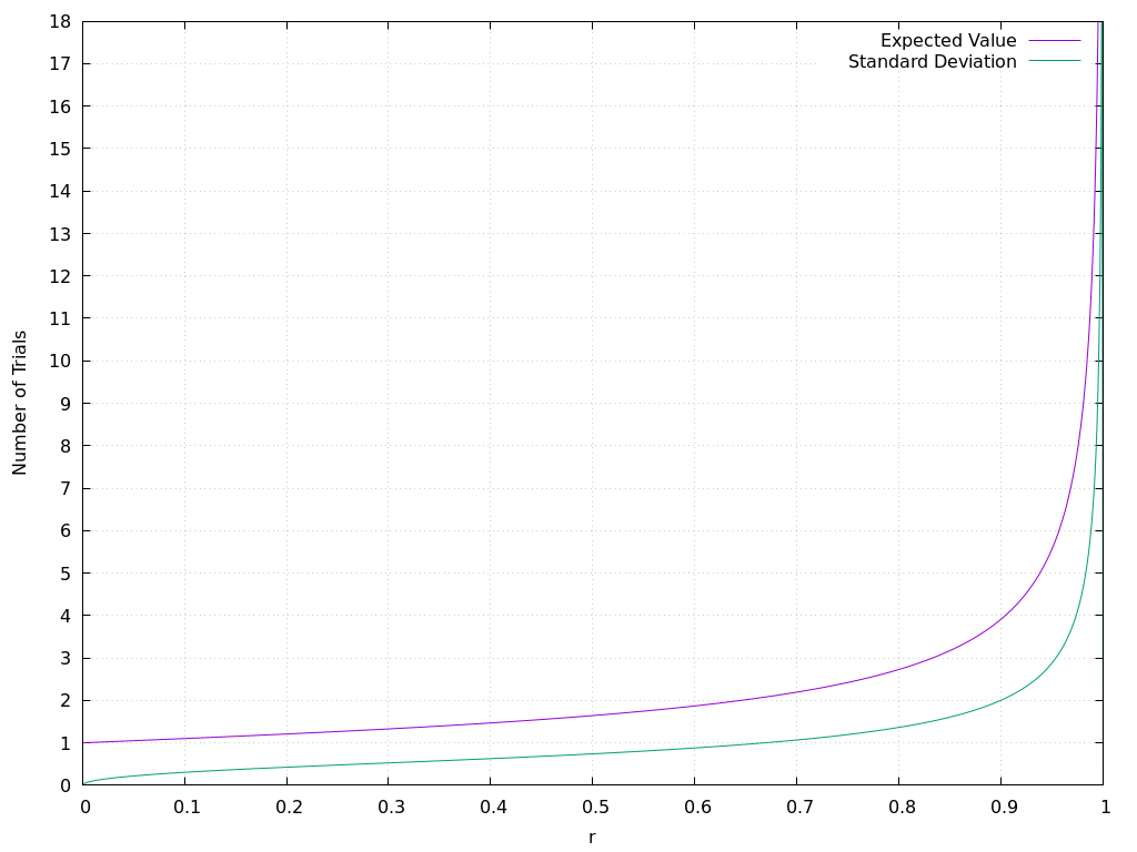
Here's a plot that displays the expected value, together with the standard deviation, for values of \(r\) between \(0\) and \(1\):

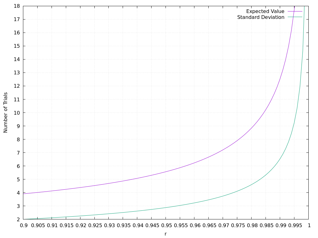
And here's the section of the plot that corresponds to the values of \(r\) from \(0.9\) to \(1\):

At the beginning, the expected value grows very slowly. But it shoots to infinity really fast when approaching \(1\).
The plots above were generated with gnuplot from the following tables:
All values are approximate, but they should suffice for most practical applications.